One of the most basic data science interview questions we are asked is about different optimization algorithms in deep learning. This article will be a one stop draft for all the information regarding optimization algorithms.

What we’ll cover?

We’ll cover the following optimization algorithms with their pros and cons:

1. Algorithms based on weight update rule.

• Gradient Descent
• Momentum Based Gradient Descent
• Nesterov Accelerated Gradient Descent

2. Batch size based optimization algorithms.

• Batch Gradient Descent
• Mini Batch Gradient Descent
• Stochastic Gradient Descent

3. Adaptive learning rate based optimization algorithms.

• Adagrad
• RMSProp
• Adam

So, without wasting much time we’ll start with our algorithms:

Algorithms based on update rule

Gradient Descent

Gradient descent is one of the most important algorithms in the machine learning world. Gradient descent helps us in finding an optimal value for weights such that the loss function value is minimum.

The equation for gradient descent is given by

Let’s understand this equation

1. Qj represents any parameter in our model.
2. α represents the learning rate i.e how fast or slow you want to update the parameters.
3. ∂J(Q)/∂Qj the derivative is to find how the cost function changes when we change our parameters by a tiny bit(also called the slope of tangent cutting at the point).

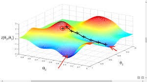
Now let’s see why gradient descent work

Let’s understand the above graph. Suppose we calculate the gradient and it comes out to be positive. Now in our equation of gradient descent(refer to figure 5), if the gradient is positive, then the value of w will decrease or move to a less positive value and vice versa for the negative gradient. Check this out using pen and paper and try to solve it.

But there is a problem with Gradient descent

Suppose during optimizing our model, we reach a point where the slope or gradient at that point is flat or Δw → 0, in this case, our update to the parameter will be very small or there will be no update. Since w = w- ηΔw.

In this case, our optimization algorithm may get stuck in the plateau region and it will slow our learning process. Vice versa on steep regions the gradient descent works very fast since the gradient is high.

So, because of this uneven optimization speed at different points on the graph, weights initialization or starting point for gradient descent algorithm can be a deciding point for how our model will perform.

But don’t worry, there is a solution to this problem and that is Momentum Based Gradient Descent.

Momentum-Based Gradient Descent.

So the one issue we found in gradient descent is that it runs very slowly on plateau regions. Momentum Based Gradient Descent handled this in a very elegant way.

Intuition: Suppose you enter a hotel and want to reach a particular room, you ask the waiter and he told you to go straight, then you asked the receptionist and she told you the way, after asking 2–3 people you become more confident about the path and started taking larger steps and finally reach your room.

So, what basically MBGD does is it keeps a record of all the previous steps that you have taken and uses this knowledge to update the weights.

The equation for Momentum Based Gradient Descent is given by:

Vₜ = γ*Vₜ-₁ + η(Δw)- (1)
wₜ₊₁  = wₜ - vₜ - (2)
combining eq 1 and 2 we get
wₜ₊₁ = wₜ - γ*Vₜ-₁ - η(Δw) -(3)
0<γ<1
if γ*Vₜ-₁ is zero, then we have our old gradient descent algo
Let's see how this works
v₀ = 0
v₁ = γ*v₀ + η(Δw₁) = η(Δw₁) (since v₀ is 0)
v₂ = γ*v₁ + η(Δw₂) = γ*η(Δw₁) + η(Δw₂)
Similarly
vₜ = γ^t-1*ηΔw₁ ..... + ηΔwₜ

I know the above equation is little bit complicated to understand, so i’ll give you a gist of it. The method above is called exponentially decaying average because we are decaying the importance of ηΔwₜ as we get further from it.

So the latest calculated gradients will have a larger impact and previous ones will have a lower impact on gradient update.

This technique is also called exponentially decaying weighted sum.

Advantage of Momentum Based Gradient Descent

• It will update quickly even on plateau regions of gradient descent graph, unlike gradient descent algorithm.

The disadvantage of Momentum Based Gradient Descent

• Due to high momentum gained, it may overshoot and take time to converge
• It oscillates in and out of the minima valley

Despite these disadvantages, it still converges faster than gradient descent.

Nesterov Accelerated Gradient Descent

In Momentum-based gradient we saw that although it converges fast still there is an overshooting problem. This problem is handled by Nesterov Accelerated Gradient Descent.

Let’s look at the equation for Momentum based gradient descent again.

wₜ₊₁ = wₜ - γ*Vₜ-₁ - η(Δw)

As you can see there are two terms getting subtracted from wₜ which leads to a large update in wₜ₊₁, which in turn leads to overshooting. So what Nesterov did is he break the above equation in two parts.

wₐ = wₜ - γ*Vₜ-₁
wₜ₊₁ = wₐ - η(Δwₐ)
vₜ = γ*Vₜ-₁ + η(Δwₐ)

We first make a temporary weight update and check whether we are close to our converging points and if not then we make the second update on the weight.

Optimization Algorithm based on Batch Size

It basically means how many examples your model actually sees before it makes an update in weight parameters. Based on batch size it can be categorized into 3 categories.

Batch Gradient Descent

In Batch Gradient Descent your model will accumulate gradients for all the training examples and then make an update in the parameters. Pseudo code for the following can be given as

X = np.arange(10) # input features having 10 examples
Y = np.arange(10) # output labels having 10 examplesfor a in range(epochs):
    for x,y in zip(X,Y):
       Δw+=calculate_grad(w,x,y)
    w = w - η(Δw)

Advantages of Batch Gradient Descent

• Batch Gradient descent can be benefited by using vectorization
• Since the weights are updated after seeing all the examples, there is less chance of noise and zig-zag movement of our gradient descent algorithm.

The disadvantage of Batch Gradient Descent

• Sometimes the size of the data could be too large to accumulate in the memory and you may need extra memory to handle it.
• Since there is less noise, there may be a scenario that it may get stuck in local minima.

Stochastic Gradient Descent

In stochastic Gradient Descent we update the parameters after each example. The pesudo code for the same is given as

X = np.arange(10) # input features having 10 examples
Y = np.arange(10) # output labels having 10 examplesfor a in range(epochs):
    for x,y in zip(X,Y):
       Δw+=calculate_grad(w,x,y)
       w = w - η(Δw)

Advantages of Stochastic Gradient Descent

• Many updates in a single pass or a single epoch.
• It is easier to fit in memory and have much less processing time.
• Due to frequent updates, there is a lot of noise introduced which may help if the gradient descent gets stuck in local minima.

Disadvantages of Stochastic Gradient Descent

• It losses the advantage of using vectorization since we are working with only one example at a time.
• Due to a lot of noise, it may take time to converge to global minima.

Mini Batch Gradient Descent

Mini Batch lies enjoy the best of both worlds. In this, we update the parameters after seeing a subset of examples.

X = np.arange(10) # input features having 10 examples
Y = np.arange(10) # output labels having 10 examples
Batch_size=2for a in range(epochs):
    count=0
    for x,y in zip(X,Y):
       count+=1
       Δw+=calculate_grad(w,x,y)
       if(count%Batch_size):
           w = w - η(Δw)

Advantages of Mini Batch Gradient Descent

• It takes advantage of vectorization, because of which the processing is fast
• The noise can be controlled by tuning the batch size

The preferred batch sizes are 32,64, 128 based on the size of dataset.

The above 3 algorithms can be used in combination with Gradient Descent, Momentum Based Gradient Descent, Nesterov Gradient Descent and the remaining that we are going to discuss.

Adaptive Learning Rate

Why do we need Adaptive Learning Rate?

In the above image suppose X1 is a sparse feature and X2 is a dense feature.

so, if write equation for gradient for w1 and w2, it will be

Δw₁ = f(x)*(1-f(x))*x1
Δw₂ = f(x)*(1-f(x))*x2Gradient Descent for w1 and w2
w1 = w1 - η(Δw₁)
w2 = w2 - η(Δw₂)

So, we can see gradients directly depend on the feature. Now if X1 is sparse then most of the elements in it will be zero. In the gradient descent algorithm, we can see that if the gradient is zero there will be no update in the parameter. So for sparse feature what we want is whenever we get any non-zero element, the learning rate should be high such that it makes a large update in w(to gain maximum information from these elements). Similarly, in the case of dense features, the parameters will update very frequently and for this we want our learning rate to be low since our Δw₂ will be high.

• We need to have different learning rates for different features in the dataset based on whether they are sparse or dense. i.e low η for dense features and high η for sparse features.

We have three algorithms that address the same problem.

• Adagrad

Adagrad works on the principle that we decay the learning rate for parameters in proportion to their update history.

The equation for Adagrad is given as

Vₜ = Vₜ-₁ + (Δw)^2 - (Eq.1)
wₜ₊₁  = wₜ - (η/√Vₜ + ε)*(Δw) - (Eq.2)

Understanding the above equation:

• Vₜ is the history term, now from equation 1 we can see that for sparse feature, Vₜ will be very small(since (Δw)² will be zero for most of the elements).
• Now, if we divide η by a small value of Vₜ, it will make a large update to wₜ₊₁(think about it!).
• Similarly, for dense features Vₜ will be a large value (since (Δw)² will be non zero for most of the elements).
• Now, if we divide η by a large value of Vₜ, it will make a small update to wₜ₊₁(since the learning rate is reduced to a small value due to division by a large value!).

But there is a problem with Adagrad

• For dense features, the value Vₜ becomes so large that it reduces the learning rate to a very small value because of which it makes the learning process for that feature very slow. This will create problems while converging to a minimum.

RMSProp

RMSProp address the problem created due to Adagrad by controlling the Vₜ parameter from exploding.

The equation for RMSProp is given by

Vₜ = β*Vₜ-₁ + (1-β)*(Δw)^2 - (Eq.1)
wₜ₊₁  = wₜ - (η/√Vₜ + ε)*(Δw) - (Eq.2)

The beta introduced controls the amount of update in the history term. Take out your pen and paper and try to think how this will work.

Adam

Adam is one of the most used optimization algorithm used in the industry. Adam is a combination of Momentum based gradient descent and RMSProp

The equation for Adam is given by

mₜ = β₁*Vₜ-₁ + (1-β₁)*(Δw)^2 - (Eq.1)
vₜ = β₂*Vₜ-₁ + (1-β₂)*(Δw)^2 - Eq.2
wₜ₊₁  = wₜ - (η/√Vₜ + ε)*(mₜ) - (Eq.3)

• mₜ is responsible for maintaining the momentum of the algorithm and prevent it from getting stuck in a plateau region.
• Vₜ is responsible for handling the adaptive learning rate

Homework for you

• There is one more step involved in Adam and this of bias correction. Do some research on this.
• Apart from above optimization algorithms there are few more which can help train your model faster. Explore those.